3D Orientation Estimation

We have developed an efficient, parallelisable computational method to determine 3D orientations at a local level. Quantifying the orientation and alignment of cells and fibres in 3D is of growing interest. Tissue function is affected by this alignment and with increases in the development and use of 3D scaffolds in bioengineering there is a need to be able determine their performance.

The algorithm performs the following steps [1]

Computes the image intensity gradients
Classifies the vectors into spherical and non-spherical using circularity testing
Computes the local orientation vectors for the identified non-spherical vectors
Assesses the distribution of the estimated local orientations over the whole volume

Image Intensity Gradients

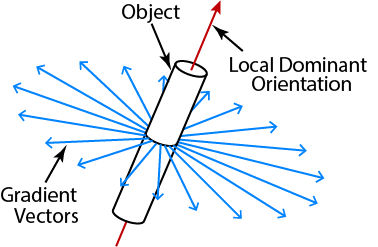
Gradient Vector Diagram — Gradient vector diagram.

Differentials of the volumetric images in each dimension $i$ are obtained via convolution $$G_i(x,y,z) = I(x,y,z)\ast h_i(x,y,z)$$ where $h_i$ is a Gaussian derivative filter to form a 3D vector field $\vec{G}(x,y,z)$.

The magnitude of $\vec{G}$ is large at object boundaries
The direction is normal to its local orientation

Therefore estimating local orientation requires estimating normal vectors to $\vec{G}$

The girdle distribution models data points in spherical polar coordinates concentrated on a great circle. The distribution is characterised by:

Concentration of points around the circle
Orientation of the polar axis

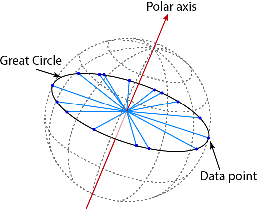
Estimating the local orientation then becomes that of determining the polar axis.

Girdle Distribution — Girdle distribution.

Our solution adapts a maximum-likelihood estimator from spherical statistics to estimate the polar axis using a local region of $\vec{G}(x,y,z)$ rather than spherical data by:

Calculating an estimator for a uniform grid of axis angles
Choosing a pair of axis angles that minimise the estimator

This method is efficient to computer, can perform the per voxel polar axis estimation in parallel and allows for a customisable search space based on the size of the grid.

Complex Statistics

Having obtained a local orientation we need to determine whether the estimate is meaningful, if the local image vectors are spherical then a local orientation angle is meaningless.

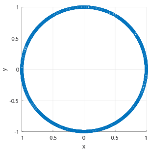
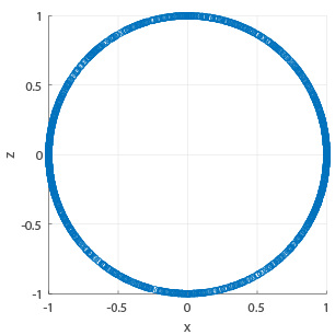
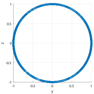
Many tests for sphericity are tailored to a particular statistical distribution or are computationally intensive. Our solution is to project the data into the 3 coordinate planes and then test for circularity.

Data which is non-circular in one or more plane is non-spherical

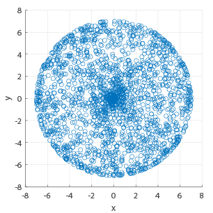
But we also need to consider not only the distribution of the angles but also the magnitude

Considering only the angles does not give all of the information
- Non-spherical data can be uniformly distributed across all angles
Using both angle and magnitude shows shows differences in the distributions

Our approach uses statistics of complex numbers to determine the circularity which takes into account both angle and magnitude and is efficient to compute.

Spherical Data — Spherical data point cloud.

Non-Spherical Data — Non-spherical data point cloud.

Non-spherical data projected onto the unit circle.

Non-spherical data point cloud.

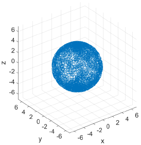
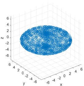
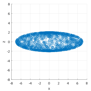
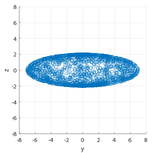
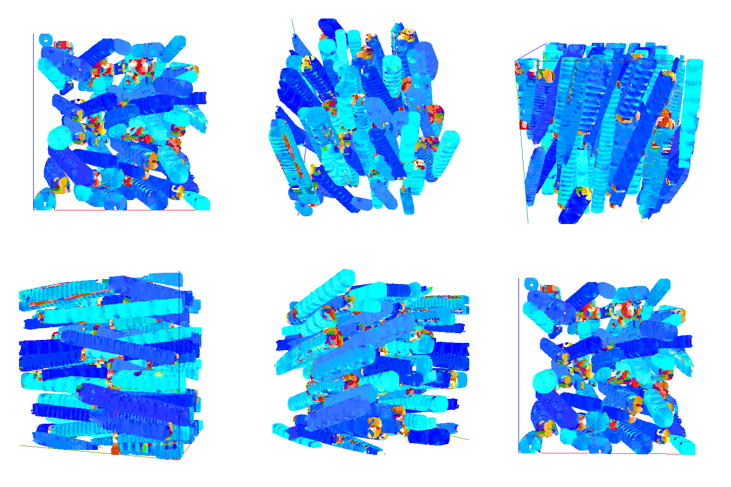
Simulated Fibres

Original Range of Angles — The original fibres.

Colour Wheel — Colour key for the different angles.

Results Range of Angles — Estimated fibres from noisy data with PSNR = 30dB.

Fibres with a range of elevation angles between 70° and 100° and azimuth angles between 90° and 120°.

Fibrous Scaffold Data

Random Scaffold Data — Random structures.

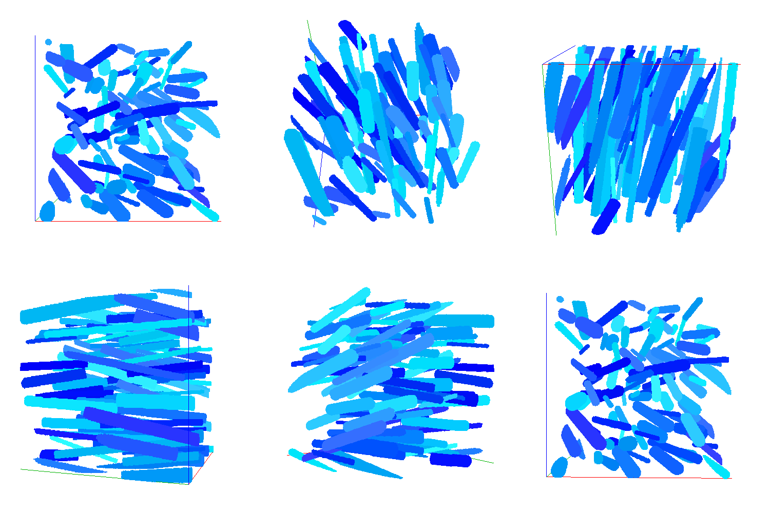
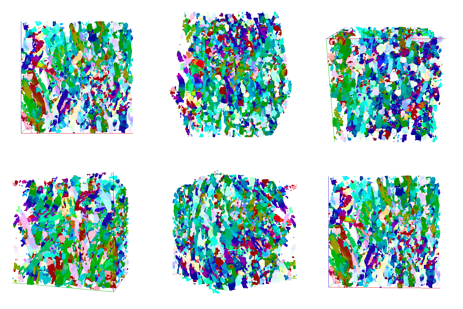
Aligned Scaffold Data — Aligned structures.

Estimated fibres from real fibrous scaffold data (datasets available here).

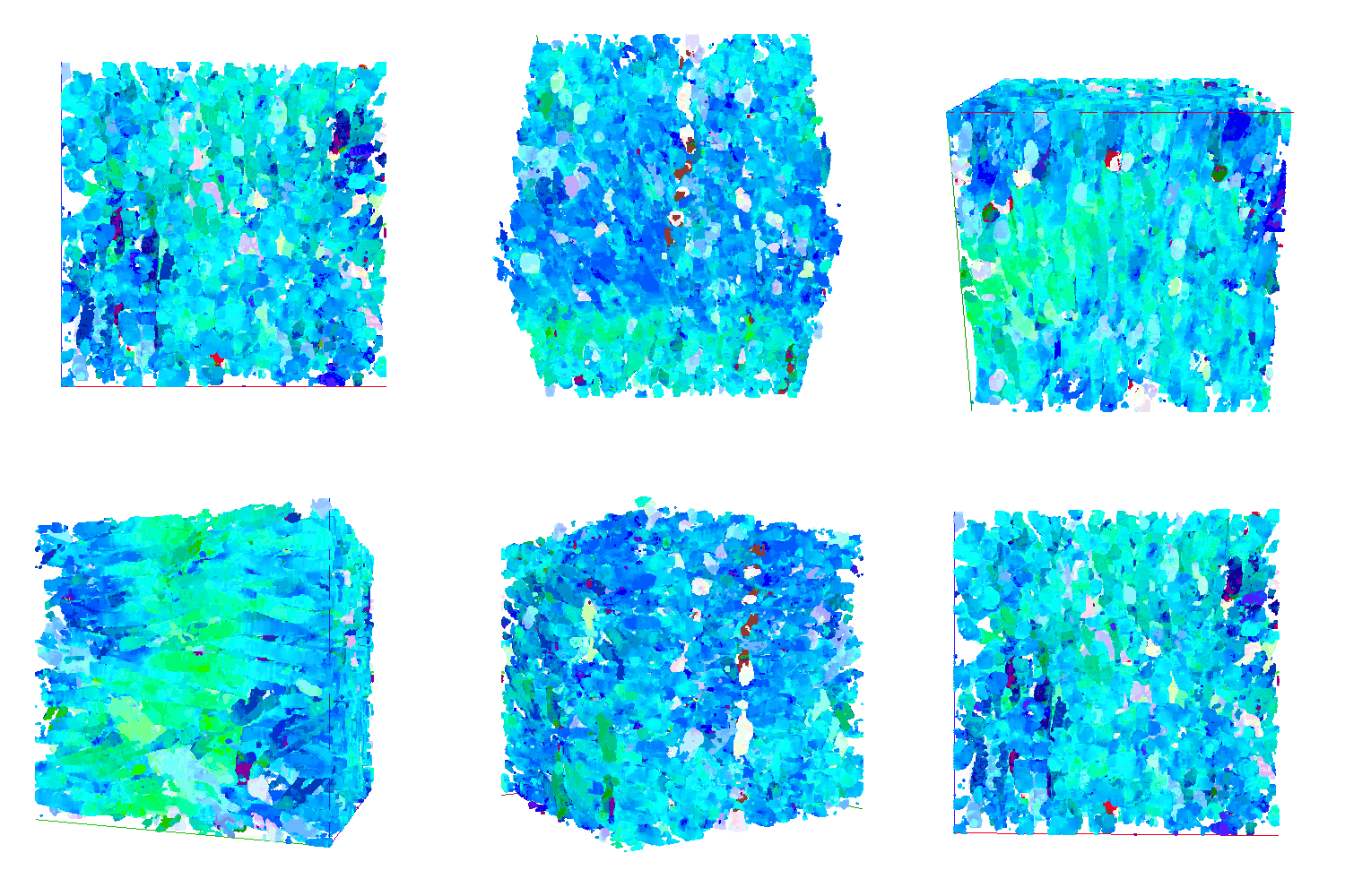
Assessing Distribution of Local Orientations

To assess the distribution of the local orientation angles across the whole volume the local orientation angles are converted to a set of unit vectors. The assessment of their distribution comprises of four measures:

The three non-circularity measures in each of the planes
- These quantify the sphericity of the overall distribution
The spherical mean resultant length $\bar{R} = \lvert\frac{1}{N}\sum_n\vec{v}_n\rvert$
- This quantifies the concentration of the vectors $\bar{R}\approx 0$ indicates the vectors are widely dispersed whereas $\bar{R}\approx 1$ indicates the vectors are heavily concentrated.

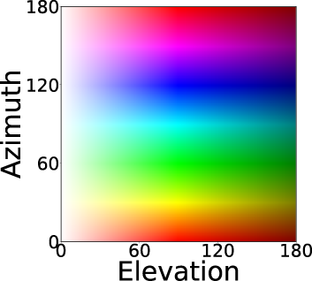
Datasets	Elevation Angles	Azimuth Angles	$\ell_{XY}$	$\ell_{YZ}$	$\ell_{XZ}$	$\bar{R}$
Single	30°--35°	70°--75°	0.83	0.94	0.94	0.96
Double	30°--35° & 110°--115°	70°--75° & 150°--155°	0.80	0.80	0.50	0.35
Range	70°--100°	90°--120°	0.64	0.80	0.51	0.89
Random	0°--180°	0°--180°	0.64	0.80	0.51	0.03
Random Scaffold Data	--	--	0.31	0.34	0.72	0.36
Aligned Scaffold Data	--	--	0.73	0.57	0.07	0.89

Assessment of the distributions of the local orientations. $\ell$ = degree of non-circularity $\bar{R}$ = spherical mean resultant length. All simulations had a PSNR of 30dB.

Code

Orientation estimation code can be found here: Orientation

References

Application of Image Processing and Circular Statistics to 3D Cellular Alignment

B. Jelfs, and C. Gilliam

In Proc. Asia-Pacific Signal and Information Processing Association Annual Summit and Conference, 2020, pp. 992–1000.

abstract html pdf code

Alignment and orientation of cells play an important part in the function of biological tissue. Recent developments in bioengineering using 3D scaffolds have created an increased need for computational techniques to measure orientation which extend beyond 2D measures to produce 3D measures of orientation. Initial studies of 3D alignment have focused on determining individual orientations, however, to truly understand the impact these structures have on the cellular alignment we need to understand the overall distribution of the orientations and their statistics. Hence, in this paper we develop an approach for determining 3D cellular alignment based on image gradients and directional statistics. The intensity gradients of the volumetric image are used to construct a 3D vector field and the local dominant orientations of this vector field then determined.